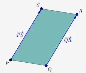
Viereck PQRS
Inhaltsverzeichnis
\(\\\)
Aufgabe 1 – Länge der Kante von P nach Q
Die Länge der Kante wird mit dem Betrag des Vektors \(\vec{PQ}\) berechnet.
\( \quad \begin{array}{ r c l } \overline{PQ} & = & \begin{vmatrix} \vec{PQ} \end{vmatrix} \\[6pt] & = & \begin{vmatrix} \vec{q} - \vec{p} \end{vmatrix} \\[6pt] & = & \begin{vmatrix} \begin{smallmatrix} \left( \begin{array}{r} -2 \\ \; 0 \\ \; 0 \end{array} \right) \end{smallmatrix} -\begin{smallmatrix} \left( \begin{array}{r} \; \; 0 \\ -2 \\ \; \; 0 \end{array} \right) \end{smallmatrix} \end{vmatrix} \\[8pt] & = & \begin{vmatrix} \begin{smallmatrix} \left( \begin{array}{r} -2 \\ \; 2 \\ \; 0 \end{array} \right) \end{smallmatrix} \end{vmatrix} \\[8pt] & = & \sqrt{(-2)^2 + 2^2 + 0^2} \\[6pt] & = & \sqrt{8} \\[6pt] & \approx & 2{,}83 \\ \end{array} \)
\(\\\)
Die Kante hat eine Länge von \(2{,}83 \, m\).
\(\\[2em]\)
Aufgabe 2 – Parallelogramm
Sind jeweils 2 Kanten parallel zueinander und gleich lang, so handelt es sich bei einem Viereck um ein Parallelogramm. Handelt es sich um ein geschlossenes Viereck, so brauchen nur 2 Kanten auf Parallelität und gleiche Länge überprüft werden. Die anderen beiden Kanten ergeben sich dann.
Die Kanten sind parallel und gleich lang, wenn die Verbindungsvektoren der entsprechende Punkte identisch sind.
Wir untersuchen die Vektoren \(\vec{PS}\) und \(\vec{QR}\).
\(\\\)
\( \quad \left. \begin{array}{ c*{7}{c} } \vec{PS} & = & \vec{s} - \vec{p} & = & \begin{smallmatrix} \left( \begin{array}{c} 1 \\ 0 \\ 4 \end{array} \right) \end{smallmatrix} -\begin{smallmatrix} \left( \begin{array}{r} 0 \\ -2 \\ 0 \end{array} \right) \end{smallmatrix} & = & \begin{smallmatrix} \left( \begin{array}{c} 1 \\ 2 \\ 4 \end{array} \right) \end{smallmatrix} \\ \\ \vec{QR} & = & \vec{r} - \vec{q} & = & \begin{smallmatrix} \left( \begin{array}{r} -1 \\ 2 \\ 4 \end{array} \right) \end{smallmatrix} -\begin{smallmatrix} \left( \begin{array}{r} -2 \\ 0 \\ 0 \end{array} \right) \end{smallmatrix} & = & \begin{smallmatrix} \left( \begin{array}{c} 1 \\ 2 \\ 4 \end{array} \right) \end{smallmatrix} \\ \end{array} \; \right\} \; \textrm{gleich} \)
\(\\\)
Es handelt sich bei dem Viereck \(PQRS\) um ein Parallelogramm.
\(\\\)
Ist an einer Ecke kein 90°-Winkel, so kann es sich nicht um ein Rechteck handeln. Wir prüfen die Orthogonalität an der Ecke des Punktes \(P\) mit der Vektoren \(\vec{PQ}\) und \(\vec{PS}\).
\(\\\)
\( \quad \begin{array}{ *{7}{c} } \vec{PQ} \circ \vec{PS} & = & \begin{smallmatrix} \left( \begin{array}{r} -2 \\ 2 \\ 0 \end{array} \right) \end{smallmatrix} \circ \begin{smallmatrix} \left( \begin{array}{c} 1 \\ 2 \\ 4 \end{array} \right) \end{smallmatrix} & = & -2 \cdot 1 + 2 \cdot 2 + 0 \cdot 4 \; = \; 2 \; \not= \; 0 \\ \end{array} \)
\(\\\)
Das Viereck \(PQRS\) ist kein Rechteck.
\(\\[2em]\)
Aufgabe 3 – Ebene E
Die Ebene stellen wir zunächst in der Normalenform
\( \quad \left( \vec{x} - \vec{p} \right) \cdot \vec{n} \; = \; 0 \)
\(\\\)
mit dem Punkt \(P\) auf. Den Normalenvektor \(\vec{n}\) berechnen wir mit dem Kreuzprodukt der Richtungsvektoren \(\vec{PQ}\) und \(\vec{PS}\) der Ebene \(E\).
\( \quad \begin{array}{ r c l} \vec{n} & = & \vec{PQ} \times \vec{PS} \\[8pt] \vec{n} & =& \begin{smallmatrix} \left( \begin{array}{r} -2 \\ 2 \\ 0 \end{array} \right) \end{smallmatrix} \times \begin{smallmatrix} \left( \begin{array}{r} 1 \\ 2 \\ 4 \end{array} \right) \end{smallmatrix} \\ \end{array} \)
\(\\\)
Dabei gehen wir folgendermaßen vor:
Die beiden Richtungsvektoren werden paarweise 2-mal untereinander geschrieben. Die erste und die letzte Zeile werden gestrichen. Dann wird über Kreuz multipliziert und jeweils die blaue Diagonale (Hauptdiagonale) minus die rote Diagonale (Nebendiagonale) gerechnet.
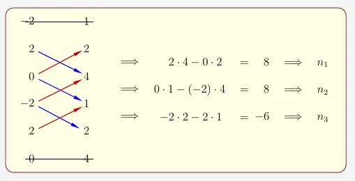
Der Normalenvektor lautet
\( \quad \begin{smallmatrix} \left( \begin{array}{r} 8 \\ 8 \\ -6 \end{array} \right) \end{smallmatrix} \\ \)
\(\\\)
Wir können die Werte halbieren. Dadurch ergibt sich ein anderer Vektor, der aber in die gleiche Richtung verläuft und auch ein Normalenvektor der Ebene \(E\) ist.
\( \quad \vec{n} \; = \; \begin{smallmatrix} \left( \begin{array}{r} 4 \\ 4 \\ -3 \end{array} \right) \end{smallmatrix} \\ \)
\(\\\)
Wir setzen in die Normalenform ein:
\( \quad \text{E} \; : \; \begin{array}{ c} \left[ \vec{x} - \begin{smallmatrix} \left( \begin{array}{r} 0 \\ -2 \\ 0 \end{array} \right) \end{smallmatrix} \right] \circ \begin{smallmatrix} \left( \begin{array}{r} 4 \\ 4 \\ -3 \end{array} \right) \end{smallmatrix} = 0 \end{array} \)
\(\\\)
Um weiter in die Koordinatenform zu kommen, lösen wir das Skalarprodukt auf.
\( \quad \begin{array}{ r c l l } \left[ \begin{smallmatrix} \left( \begin{array}{r} x_1 \\ x_2 \\ x_3 \end{array} \right) \end{smallmatrix}- \begin{smallmatrix} \left( \begin{array}{r} 0 \\ -2 \\ 0 \end{array} \right) \end{smallmatrix} \right] \circ \begin{smallmatrix} \left( \begin{array}{r} 4 \\ 4 \\ -3 \end{array} \right) \end{smallmatrix} & = & 0 & \\[10pt] \begin{smallmatrix} \left( \begin{array}{l} x_1 \\ x_2 + 2 \\ x_3 \end{array} \right) \end{smallmatrix} \circ \begin{smallmatrix} \left( \begin{array}{r} 4 \\ 4 \\ -3 \end{array} \right) \end{smallmatrix} & = & 0 & \\[10pt] x_1 \cdot 4 + (x_2 + 2) \cdot 4 + x_3 \cdot (-3) & = & 0 & \\[6pt] 4x_1 + 4x_2 + 8 -3x_3 & = & 0 & | -8 \\[6pt] 4x_1 + 4x_2 -3x_3 & = & -8 \\ \end{array} \)
\(\\[2em]\)
Aufgabe 4 – Schnittpunkt
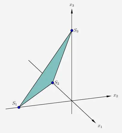
Der Schnittpunkt mit der \(x_3\)-Achse ist der Spurpunkt \(S_3(0|0|x_3)\) der Ebene \(E\).
\(\\\)
Mit \(x_1=0\) und \(x_2=0\) eingesetzt in die Ebene \(E\) erhalten wir
\( \quad \begin{array}{ r c l l } 0 \cdot 4 + 0 \cdot 4 - 3x_3 & = & -8 & \\[8pt] -3x_3 & = & -8 & | : (-3) \\[8pt] x_3 & = & \frac{8}{3} \\ \end{array} \)
\(\\\)
den Spurpunkt \(S_3\left(0|0|\frac{8}{3}\right)\) der Ebene \(E\).
Die Wand befindet sich senkrecht über dem Koordinatenursprung in einer Höhe von
\( \quad h \; = \; \frac{8}{3} \; \approx \; 2{,}67 \; m \)
\(\\[2em]\)
Aufgabe 5 – Punkt mit ganzzahligen Koordinaten
Wir setzen \(x_3=2\) in Ebene \(E\) ein.
\(\\\)
\(\quad \begin{array}{ r c l l } 4x_1 + 4x_2 - 3 \cdot 2 & = & -8 & \\[6pt] 4x_1 + 4x_2 - 6 & = & -8 & | + 6 \\[6pt] 4x_1 + 4x_2 & = & - 2 & | - 4x_1 \\[6pt] 4x_2 & = & - 2 - 4x_1 & | : 4 \\[6pt] x_2 & = & - 0{,}5 - x_1 \\ \end{array} \)
\(\\\)
Wir probieren verschiedene Werte für \(x_1\) :
\(\\\)
\( \quad \begin{array}{ r | l | r } \mathbf{x_1} & \mathbf{\text{Rechnung}} & \mathbf{x_2} \\[6pt] \hline -3 & - 0{,}5 - (-3) & 2{,}5 \\[6pt] -2 & - 0{,}5 - (-2) & 1{,}5 \\[6pt] -1 & - 0{,}5 - (-1) & 0{,}5 \\[6pt] 0 & - 0{,}5 - 0 & - 0{,}5 \\[6pt] 1 & - 0{,}5 - 1 & - 1{,}5 \\[6pt] 2 & - 0{,}5 - 2 & - 2{,}5 \\[6pt] 3 & - 0{,}5 - 3 & - 3{,}5 \end{array} \)
\(\\\)
Es ist zu erkennen, dass wir für \(x_2\) immer eine Zahl mit einer Nachkommastelle bekommen, wenn wir für \(x_1\) einen ganzzahligen Wert einsetzen. Folglich gibt keinen Punkt, bei dem sowohl \(x_1\) als auch \(x_2\) ganzzahlig sind.
\(\\\)